But you may be wondering how to format tracking numbers in Excel if you need those numbers ot stop converting to scientific notation. Our tutorial below will show you a formatting option to use which can give you the desired formatting you need.
How to Format Tracking Numbers in an Excel Shipping Spreadsheet
Our guide continues below with additional information on how to format Excel tracking numbers, including pictures of these steps. Many large businesses will ship dozens, if not hundreds or thousands of packages in a day. Almost all of the customers receiving those packages will want a way to track their shipments, so you may find yourself in possession of an Excel file with a lot of tracking numbers. But Excel has an annoying habit of displaying large numbers, such as tracking numbers, as scientific notation when the number is wider than the column in the spreadsheet. While these formatting options can be useful when you need to do things like convert text in a cell into numbers, they can also be problematic at times. Fortunately you can resolve this problem by expanding the column or, if that doesn’t work, by changing the format of the cells. If you are looking for a fast way to fix all o the column widths and row heights in your worksheet, then our Excel autofit all columns guide can show you how.
How to Display Full Tracking Numbers in Your Cells in Excel 2013 (Guide with Pictures)
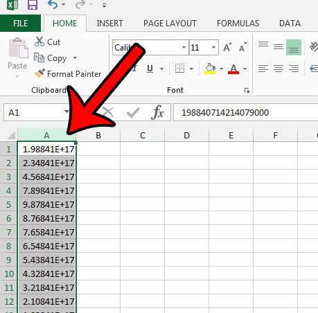
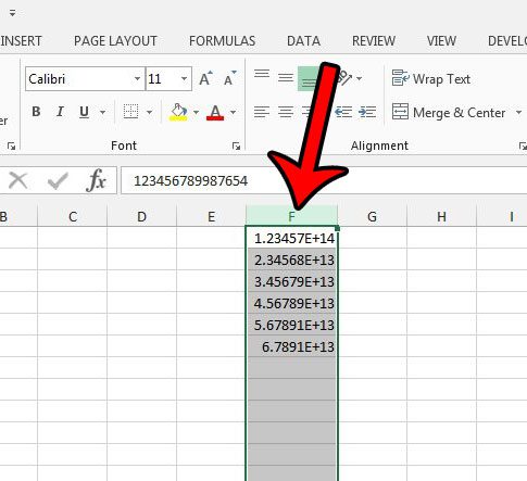
The steps below will assume that you have a spreadsheet full of tracking numbers, and that they are all displaying as scientific notation. This means that they are probably in a format like 1.23456E+7, or something similar. There are two potential ways to resolve this issue. We will show you both ways as one long method, but you may find that the first part, which consists of making the column wider, is enough to fix the issue. If that is the case, then you can just stop at that point.
Step 1: Open the spreadsheet containing the tracking numbers that are currently displaying as scientific notation.
Step 2: Click the column letter containing the tracking numbers that are displaying incorrectly. If the tracking numbers are in a row instead, click the row number.
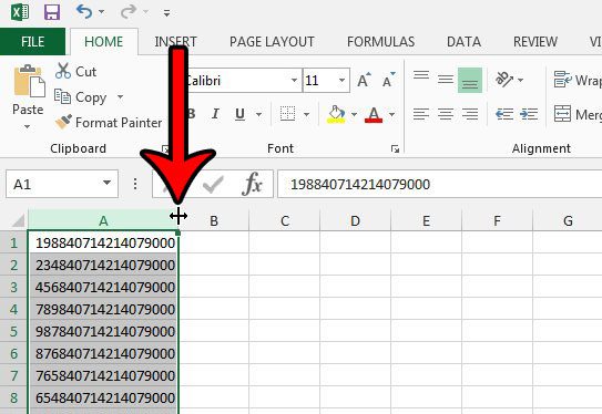
Step 3: Position your mouse on the right border of the column heading (the cursor should change to look like a vertical line with an arrow coming out of either side), then double-click your mouse to automatically resize the column to fit the width of your tracking numbers.
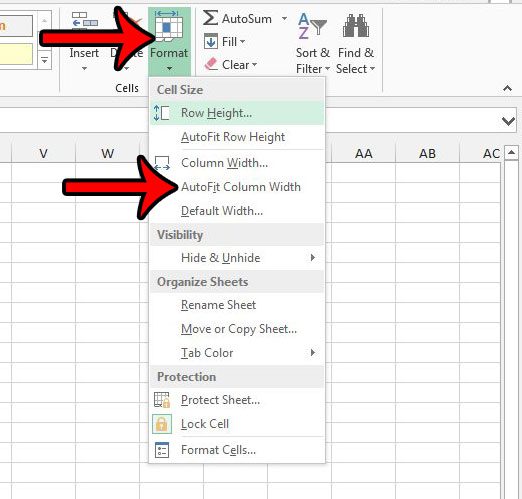
If you are having difficulty doing it this way, you can also autofit the column by clicking the Format button in the Cells section of the ribbon, then clicking the AutoFit Column Width option. If automatically resizing the column didn’t do anything, then your cells might not be in the right format, so continue with step 4 below.
Step 4: Select the column with the scientific notation numbers again.
Step 5: Right-click on the selected cells, then click the Format Cells option.
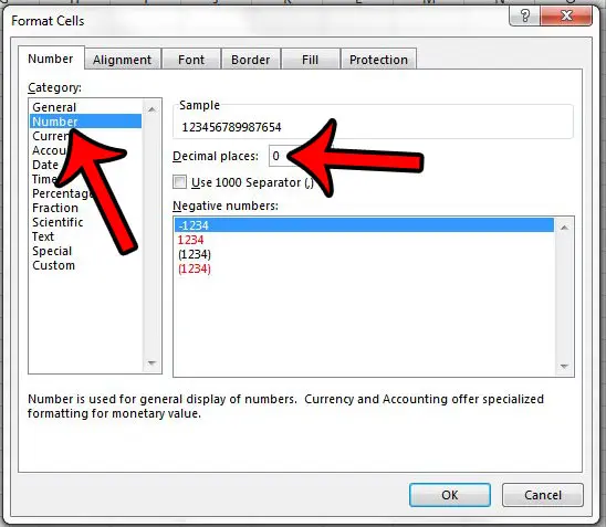
Step 6: Select Number under the Category section at the left side of the window, change the value in the Decimal places field to 0, then click the OK button.
The full tracking numbers should be visible now. If you see a series of #######, then perform the first three steps of this guide again to expand the column width. Do you need a quick way to remove the last digit from a series on cells in your spreadsheet? I have to do this a lot when I create barcodes, since a lot of barcode formats use something called a “check digit” that is calculated automatically. Learn how to do this with a formula and save yourself the tedious task of doing it manually.
Additional Sources
After receiving his Bachelor’s and Master’s degrees in Computer Science he spent several years working in IT management for small businesses. However, he now works full time writing content online and creating websites. His main writing topics include iPhones, Microsoft Office, Google Apps, Android, and Photoshop, but he has also written about many other tech topics as well. Read his full bio here.
You may opt out at any time. Read our Privacy Policy
