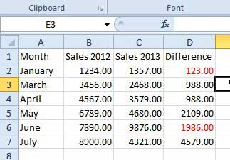
When dealing with large spreadsheets in Excel 2010, it is important to be able to identify the information that is more important than the rest of the information. In some cases, such as a budget or a sales report, this could be situations where sales have decreased, or expenses may exceed income. Excel will handle negative numbers by placing a “-” sign in front of them, but you may find that this is not enough. Fortunately, you can also adjust the formatting in your spreadsheet so that the numbers are automatically displayed with a red font.
Microsoft Excel – How to Make Negative Numbers Red
Our guide continues below with another way to format negative numbers as red, including pictures of those steps.
How to Automatically Format Negative Numbers with Red Text in Excel 2010 (Guide with Pictures)
Of course, you could always go through and manually change the color of the text to red, but that is both tedious and prone to potential mistakes. The method described below is simple and automatic, and you can even choose to apply it to your entire worksheet so that additional negative number entries are formatted correctly. So continue reading below to learn how to make negative numbers red in Excel 2010.
Step 1: Open your worksheet in Excel 2010.
Step 2: Highlight the cells containing the information that you want to format with the automatic red font for negative numbers.
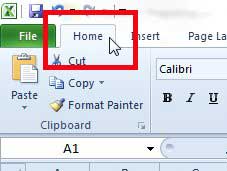
Step 2: Click the Home tab at the top of the window.
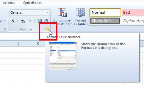
Step 3: Click the Format Cells: Number button at the bottom-right corner of the Number section of the ribbon.
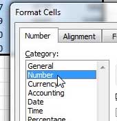
Step 4: Select the Number or Currency option from the list at the left side of the window.
Note that choosing the currency option will place a $ sign in front of any number in the spreadsheet.
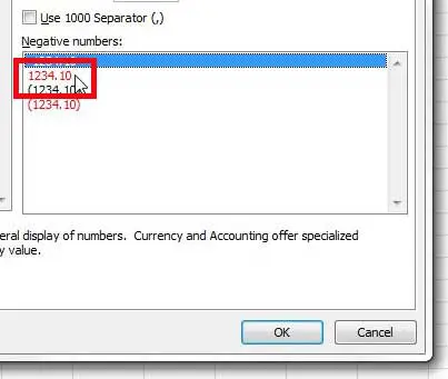
Step 5: Select the 1234.10 option under Negative numbers, then click the OK button.
When you return to your spreadsheet you will notice that all of your negative numbers are now displayed in red, like in the image below.
Our tutorial continued below with more information on red number formatting for negative numbers, including another way you can do it, plus some ways to customize this formatting option.
How to Open the Format Cells Dialog Box
In the sections above we discussed two different ways that you could switch to red negative numbers. Both of these options take you to the Format Cells window. Which option you use to open that window is up to you, but both allow you to achieve the same result. To recap, these methods are: Another Excel tool you may want to consider for accomplishing formatting like this, or other types of results, is called “Conditional Formatting.”
How Do I Use Conditional Formatting in Excel?
You may have encountered information about conditional formatting when you were trying to figure out how to make your negative numbers red. When you apply conditional formatting to a cell or range of cells you are telling Excel to apply formatting only under certain conditions. One of these conditions can be defined by creating a custom format that keeps positive numbers at their default display, while making negative values red or some other color. To test this out you can select a group of cells, at least one of which should have a negative cell value. You can then click the Home tab at the top of the window, then click the Conditional Formatting button in the Styles group of the ribbon. If you select the Highlight Cells Rules option then pick the Less Than option, a new Less Than dialog box will open. If you enter “0” into the Format cells that are Less Than option, you can click the drop down list next to “with” and choose the Red Text option, one of the other available options, or even the Custom Format option. When you are done click the OK button.
More Information on How to Make Negative Numbers Red in Excel 2010
While the steps in this article are focused on showing negative numbers in red in Excel 2010, they will also work in most other versions of Microsoft Excel. For example, if you want to know how to make negative numbers red in Excel 2013 then you could select the whole sheet, right-click a cell and choose Format Cells, then select the Number option and click the red numbers under the Negative numbers section. Using the right-click option from the paragraph above and choosing the Format Cells option will also work in Excel 2010, and can be a quicker way to open the Format Cells dialog box if you are comfortable with right-clicking. If you want to apply this formatting to the entire worksheet, rather than just a small cell range of data, then you can either click the gray cell above the row 1 heading and to the left of the column A heading, or you can press the keyboard shortcut of Ctrl + A. Either of these methods offers a quick way to select all of the cells in a worksheet. If you go with the Format Cells window option instead of creating a conditional formatting rule or a custom number format, then you will be able to select whether you want your negative numbers to have a minus sign in front of them or not. It can be useful to keep the negative sign there, especially if other people that are viewing or editing the spreadsheet might not be familiar with custom number formats. If you are printing a spreadsheet that is not going to fit on just one page, then it will be helpful to your readers if you re-print the column headers at the top of every page. Read this article to learn how.
Additional Reading
After receiving his Bachelor’s and Master’s degrees in Computer Science he spent several years working in IT management for small businesses. However, he now works full time writing content online and creating websites. His main writing topics include iPhones, Microsoft Office, Google Apps, Android, and Photoshop, but he has also written about many other tech topics as well. Read his full bio here.
You may opt out at any time. Read our Privacy Policy

